
Automatic control, particularly the application of feedback, has been fundamental to developing automation.
The origins of automation began in the ancient world with level control, water clocks, and pneumatics/hydraulics. From the 17th century onwards, systems were designed for temperature control, regulating steam engines, and the mechanical control of mills. Then, the 19th century saw the emergence of unstable feedback systems where the value of a controlled object can go to infinity. A stability criterion surfaced independently towards the end of the century by Routh in England and Hurwitz in Switzerland. The 19th century, too, saw the development of servomechanisms, first for ship steering and later for stabilization and autopilots. As aircraft were invented (literally), however, instability gained a new dimension.
In the 1920s, Minorsky’s theoretical analysis of ship control clarified the nature of three-term control, also being used for process applications. Based on servo and communications engineering developments of the 1930s and driven by the need for high-performance gun control systems, the coherent body of theory known as ‘classical control’ emerged during and just after WW2 in the US, UK, and elsewhere, as did cybernetics, or the study of controls used in technology (e.g. auto-pilot, maintaining room temperature, and more).
Meanwhile, an alternative approach to dynamic modeling had been developed, based on the approaches of Poincaré and Lyapunov. Information was gradually disseminated, and ‘state-space’ or ‘modern control’ techniques, fueled by demands of missile control systems, then the digital computer opened possibilities for automatic control and optimization.
Automatic controls, both classic analog and modern digital systems, have greatly improved the process operation safety, stabilities and efficiencies for the process industries such as oil refining, chemical, and petrochemical. However, a plant’s maximum economic potential couldn’t have been realized until the invention of the Multivariable Model Predictive Control (MPC) technology. As an example, historically, the various type of furnaces’ operation and control have not minimized energy use and carbon emissions but since MPC that is changing!
Model Predictive Control (MPC) differs from traditional control techniques in that process models are used to determine the control actions. As a result, the controller can predict the future behavior of the process, greatly enhancing the control system’s stability and accuracy. When the MPC is extended to the Multivariable System, the optimal solution based on the economic functions is then possible.
As such an MPC technology, PACE (Platform for Advanced Control and Estimation) is an advanced software package. As one of its unique features, PACE’s economic functions make it outstanding in MPC applications. It’s comprehensive in that for a complex process, multiple math equations involving both MVs (manipulated variables) and CVs (controlled variables) can be used to define a controller’s optimization, and these multiple economic equations can also be prioritized. It’s flexible in that in PACE Run Time, the economic functions can be tuned and selectively turned on and off.
Figure 1 shows the PACE application for the naphtha split column in a refinery, after the controller initiates the design time simulation:

Figure 1. PACE application for the naphtha split column in a refinery
Figure 2 demonstrates two economic functions for optimal control. One function involves minimizing reflux while the other is to maximize naphtha products with the same priority:

Figure 2: Two economic functions for optimal control
Once the controller is turned on, the economic functions lowered the reflux until the reflux to feed ratio CV NSU_RR is pushed to its low limit and raised the hot oil flow until the second tray temperature reaches its high limit as illustrated in Figures 3 and 4.
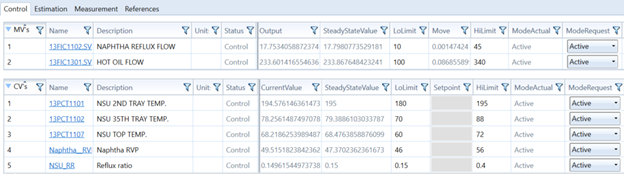
Figure 3: Control panel pushed to low limits

Figure 4: Economic functions
We recommend the economic function not be turned on right away when the controller is put online and turned on for closed-loop control, this could allow the controller to get all the CVs in the proper range for optimization as shown in Figure 5.
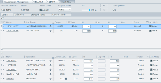
Figure 5: Coefficient of variation in the proper range for optimization
Once the economic functions are turned on, in this case, to minimize the reflux and maximize overhead product yield, the controller immediately calculated the MV moves such as reducing the reflux and increasing the hot oil flow, to push two CVs to the high limits as depicted in Figure 6.

Figure 6: Two coefficient of variation reach high limits
The engineer could observe the online MVs and CVs trend and make changes in the necessary tuning parameters, such as steady state deviation, steady state priority, dynamic X factor, and more in the economic function to improve the controller performance, as shown in Figures 7 and 8.
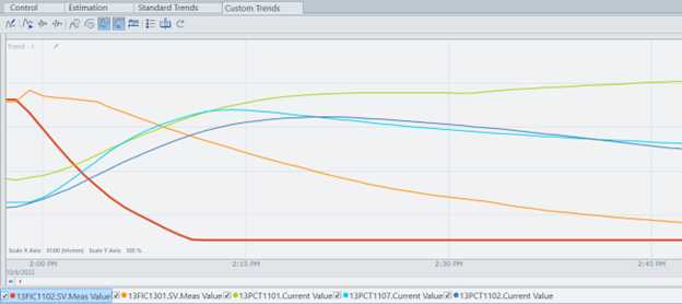
Figure 7: Graph demonstrating controller performance

Figure 8: Dashbaord showing tuning parameters
PACE can be applied to wide range of industry processes for optimal control. Its multiple economic functions design and flexible tuning parameters in real time control make it a powerful tool in maximizing plants’ production and yield, minimizing energy consumption and carbon emissions.
For more information how PACE advanced technology can help you optimize your control processes, please contact Brian Burgio, Program Manager.